VLOOKUP and HLOOKUP are the go-to functions for most Microsoft Excel users to look up data in a table. However, there exists an alternative approach that not only accomplishes the same task but also offers additional advantages – the powerful combination of INDEX and MATCH functions. Utilizing these two formulas together provides enhanced flexibility when seeking specific data.
The idea behind INDEX & MATCH is straightforward. The INDEX function is used to locate the data reference, while the MATCH function scans an array (single-dimensional) for the desired value and returns its coordinates as a numerical value. These numerical coordinates then serve as inputs for the INDEX function, seamlessly facilitating the retrieval of the desired data.
In this article, we will show some examples for how to use this dynamic duo using a downloadable workbook template. Feel free to access the spreadsheet template provided here to follow along with the examples discussed.
INDEX Function
The INDEX function is a great function for extracting data from a specified range. Its syntax is straightforward:
=INDEX(array, row_num, [column_num])
Parameters:
- array: the look up table
- row_num: row coordinate
- column_num: column coordinate (optional)
For example, the INDEX formula below will return the value in the 4th row and 3rd column in the A2:C6 range,
=INDEX(A2:C6,4,3)

INDEX function can work with single dimensional ranges without an column_num argument. The same goes for horizontal single dimensional ranges. Here is an example for a vertical single dimensional range,
=INDEX(C2:C6,4)

Below is an example for a horizontal range,
=INDEX(A5:C5,3)

MATCH Function
The MATCH function, with its three arguments, is a powerful tool for locating values within a range.
=MATCH(lookup_value, lookup_range, [match_type])
Parameters:
- lookup_value: what you want to look up
- lookup_range: where you are looking
- match_type: match type (optional)
While lookup_value and lookup_range are pretty self-explanatory, match_type can be confusing at first. This parameter essentially works like VLOOKUP and HLOOKUP’s range_lookup and tells Excel to do an exact, or an approximate match. However, instead of range_lookup’s 2-option TRUE/FALSE values, match_type can have three values (-1, 0, and 1).
| Value | Match Type | Behavior |
| 1 or omitted | Approximate | MATCH finds the largest value less than or equal to lookup value. Lookup array must be sorted in ascending order. |
| 0 | Exact | MATCH finds the first value exactly equal to lookup value. Lookup array does not need to be sorted. |
| -1 | Approximate | MATCH finds the smallest value greater than or equal to lookup value. Lookup array must be sorted in descending order. |
Although match_type is optional and your MATCH function will work just fine without it for approximate searches, it is a good practice to always enter a value here. Trying to search an exact value without arguments can give you the wrong results.
Let’s look at an example again. The formula below can give us the position of the employee name entered into B8,
=MATCH(B8,A2:A6,0)

To look for the department position,
=MATCH("Department",A1:C1,0)

INDEX and MATCH Combination
Now, let’s combine the two functions. To break it down,
=INDEX(table you are looking,
MATCH(what you want to look up, where you are looking, match type),
MATCH(what you want to look up, where you are looking, match type)
)
If either the row or column coordinate has a static value, you can replace that value with one of the MATCH functions, which in this case is redundant. Combining the two examples from before, let’s look for the employee’s department.
=INDEX(A2:C6,MATCH(B8,A2:A6,0),MATCH(A9,A1:C1,0))
The formula above will highlight these ranges,
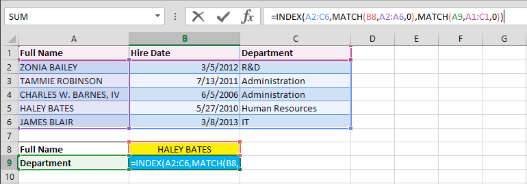
Searching for ‘Haley Bates’ gave us ‘Human Resources’ as her department.

Advantages of Using INDEX and MATCH Combo
INDEX and MATCH Offers 2-way Lookup
VLOOKUP can only search from left to right, whereas INDEX & MATCH combination allows it to overcome this limitation and look up data both left to right and right to left.
Performance of INDEX and MATCH
Although this may not mean much for casual Excel users, VLOOKUP drastically slow down complicated data models. INDEX and MATCH offer better overall performance.
The combo is a lifesaver when working with array formulas that perform multiple actions with a single formula.
No Issues When Inserting or Deleting Columns (or Rows for HLOOKUP)
If column index number (3rd argument of VLOOKUP and HLOOKUP) wasn’t been set dynamically, it’s usually not a good idea to delete or move a column in the lookup table. Plus, setting column index number dynamically means that you’re going to be needing another formula inside VLOOKUP. Yeah, you’re not dealing with a single formula anymore in this case.
The INDEX & MATCH alternative is a safer bet if you think you’re going to be inserting or deleting columns. This becomes a great advantage when working with large datasets that require frequent updates.
No 255-Character Limit for a Lookup Value's Size
Both VLOOKUP and MATCH are limited to 255 characters for lookup criteria. However; INDEX & MATCH combo make this search viable with a little tweak. For example, if lookup value (E2) exceeds the 255 character limit, a modified version of INDEX and MATCH combination can be used (Here we are searching in the range A2:B6),
=INDEX(A2:B6,MATCH(TRUE,INDEX(A2:A6=E2,0),0),2)

INDEX, MATCH combination provides Excel users an efficient and flexible data retrieval way, offering solutions to common challenges faced in spreadsheet analysis.
In summary, the combination of the INDEX and MATCH functions in Excel represents a powerful and dynamic tool for data retrieval, offering an efficient solution to many of the challenges commonly encountered in spreadsheet analysis. This pairing surpasses the limitations of more traditional lookup methods, such as VLOOKUP, by providing greater flexibility in how data is searched and retrieved. With the ability to look up values in any column and return corresponding data from any row, INDEX & MATCH give users the freedom to navigate through their spreadsheets with precision and customization. This flexibility is particularly beneficial in handling large datasets where data structures may not be conducive to simpler lookup functions. Furthermore, the use of INDEX and MATCH enhances the accuracy and efficiency of data analysis, allowing for more complex and nuanced data interrogation without the need for cumbersome workarounds.