Merge Columns
Traditional Copy+Paste might do all you want, but when working with large tables that are constantly updated, it's a tedious task to merge columns of data. To merge two columns in excel, you can use a formula combination that will save you time and prevent errors.
Syntax of the Merge Columns Formula
To merge two columns in excel, you can easily use the formula below:
=IFERROR(
INDEX(first list, ROWS(expanding range from 1st row)),
IFERROR(
INDEX(second list, ROWS(expanding range from 1st row) - ROWS(first list)),""))
Step by Step
To apply the merge columns formula;
- We need to wrap the entire formula set inside a =IFERROR( so that the calculation will continue with the second list after all items from the first is
- Use the INDEX function to get values from the first list (i.e., INDEX($B$2:$B$5,ROWS(F$1:$F1)))
- Use another IFERROR( to return empty values instead of errors
- Use the INDEX function again to get values from the second list (i.e., INDEX($D$2:$D$7,ROWS(F$1:$F1)-ROWS($B$2:$B$5)))
- Finish the formula with the second argument of IFERROR ""))
- Copy down the formula to the remaining rows as necessary
How to do it?
The merge columns formula combination will start with the first list to get values and return errors once no more items are in the first list.
INDEX($B$2:$B$5,ROWS($F$1:F1))
If there is an error, the formula will move on to the values from the second list. We must subtract the first list item count from our incremental index number.
INDEX($D$2:$D$7,ROWS($F$1:F1)-ROWS($B$2:$B$5))
If the second list ends, the formula will return empty cells ("") to hide the errors.
Let's take a look at the ROWS functions here. The ROWS function returns the count of rows in a specified range. So, in a dynamic range like $F$1:F1, updating it to $F$1:F2 will return an incremental number with each row because the range in the ROWS function expands.
The INDEX function needs an index number starting from 1 for the second list. To do this, the auto-incremental ROWS formula value should be subtracted from the first list item count. The first list range must be absolute so that it won't return different values (i.e., ROWS($B$2:$B$5)).
Alternatively, the COLUMNS function can be used to merge two horizontal lists.
=IFERROR(
INDEX($B$2:$B$5,ROWS($F$1:F1)),
IFERROR(INDEX($D$2:$D$7,ROWS($F$1:F1)-ROWS($B$2:$B$5)),""))
If you still have issues, don't hesitate to contact Microsoft for official support or ask the community. Mastering the art of merging columns in Excel is now within your grasp. Click here to learn how to merge cells in Excel without losing your data.