Excel charts are one of the most used and easy to understand data visualization tools. Excel provides many chart types as well as numerous personalization options. One of the cool features is the ability to change number format in Excel chart.
Steps
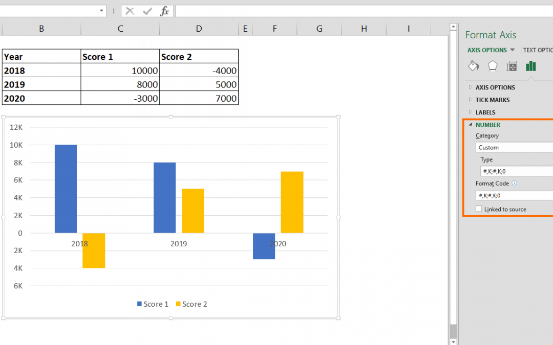
- Double-click on the value-axis that you want to modify
- Make sure that AXIS OPTIONS is active at the right panel side
- Expand NUMBER section
- Select a preset number format or Custom in Category dropdown
- Type your custom number format code into Format Code textbox
- Click Add button to apply number format
How
In Excel, you can apply any number format on value-axis values as you can apply them to cells that contains numbers. The important point here is that a number format can be applied to values-axis only. This is mainly because value-axis contains numbers or date/time values which are numbers for Excel as well.
Most charts like bar and line charts have single value-axes. On the other hand, Scatter and Bubble charts have 2 value-axes that you can format both individually.
Additionally, if you need to create and apply your custom number formats, please refer our guide for custom number formats: Number Formatting in Excel – All You Need to Know