Excel’s Pivot Tables are very powerful in the sense that you can perform most data organization and analysis tasks on the fly. Although Pivot Tables have several advantages over using formulas for the same effect, working with Pivot Tables can be tricky in certain scenarios. In this guide, we’re going to show you how to create data tables using formulas as Pivot Table alternative. For more information about Pivot Tables please see Data Analysis in Excel.
Pivot Tables are essentially user-interface helpers that can summarize and present data in a table format. The family of “…IFS” functions can mimic this same behavior through a series of formulas. Functions like SUMIFS, COUNTIFS and AVERAGEIFS that are available in Excel 2007 or newer, support using multiple criteria as parameters. If you are using Excel 2016 or newer, you can also add MAXIFS and MINIFS functions to the mix. Briefly, you can use the “…IFS” functions to achieve the same results of a Pivot Table with a little bit of ground work. Let’s see how this works on an example. You can download our workbook below.
Sample Case
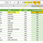
Our sample workbook contains a Pivot Table that sums all values under the Total column and filters them by the Type and Generation columns. While the column Type is used as the row headers for the Pivot Table, the column Generation represents the column headers. For example, the value 1165 is the sum of Total values for Type = WATER and Generation = I.

Creating a Table Layout
Row and column headers
When you set a field as a row or column, a Pivot Table populates the cells with a list of distinct values of those fields (column). You need to do this step by manually. We're going to use Excel's Remove Duplicates feature to get a list of distinct values for our Pivot Table alternative.
Select the cells under the column Type, then copy and paste them into the range which will be the rows of the table. When the copied cell range is selected click the Remove Duplicates button under the DATA tab in the Ribbon.

Repeat the same process for the column Generation. You also need to place these values as column headers. To do this, you can transpose the values using special paste.

Alternatively, you can use formulas to generate a list of distinct values. If the fields are going to remain static, the formula approach will probably take longer. To learn more about other ways to find unique values see: How to find unique values Excel.
Formatting and grand totals
Next, we’re going to apply formatting to make the table easier to read. In this example, we applied background colors and borders to make our table look like a regular Pivot Table.
We also added grand totals to the bottom of the table area. We’ve created this table for the purpose of showing the totals, and added SUM functions to add the values from both the rows or columns.

Adding the Formulas
Finally, we’re going to add other formulas to allow for better insight of the data. An “…IFS function” can consolidate the data through range-value pairs for certain criteria. Below is an example.
You need to use criteria range-criteria pairs for all fields that you want include as criteria. Since we are using two fields as criteria (Type and Generation) in this example, we included two pairs in the formula:
Notice the “$” characters in the references. These are used to lock the following row or column when copying formulas and make them “absolute references”. For example, the values from the column Type are listed vertically, and assume that we want the column references to remain the same when copying. To do this, we’re using a $ character before the column letter, T. The $ character is placed before the row number for the criteria reference, 3.
Copy the formula for the other cells to complete the table calculations.

As useful they might be, Pivot Tables are not your only choice for creating data tables. In some cases, using formulas instead can actually end up being easier, or allow you to add more functionality.