Let’s take a look at how we can create a spreadsheet that will allow our customers to filter through all this data to find the product they are looking for. In this example, we are going to be using a pricing list for a liquor store. We have a long list of spirits that are each of a different size, brand, type, and cost. Press the button below to download the spreadsheet template.

In order to create a funneling selection mechanism, we’re going to need to setup dynamic lists which will update based on user selection. From top to bottom we have Description, Brand, Size, and Price. Let’s begin by creating a user input area where these parameters will be set.

Concatenating the List
Here, we decided to create a form structure where users can make selections at each row to narrow down the results. The first level, Description has no other dependencies, meaning that all options listed here will be available regardless of other selections. We’re going to add this selection first.
A product price can only be reached after going through 3 levels of selections. After the Description list, we need to generate 2 unique columns for 2 other dependencies, Brand and Size. While concatenating Description & Brand values is enough for the Brand selection, we’re going to need to concatenate all three remaining properties, Description & Brand & Size, for Size.

Create Distinct Values List
We begin by creating lists of distinct values from applicable columns by removing duplicates. Follow the steps below to do this.
- Copy Description, Brand and Size columns to another sheet. Here we named the new tab
- Select all values for the Description

When you’re ready, press Remove Duplicates button under the Data tab.

Make sure you select Continue with the current selection option, otherwise values from adjacent columns will be removed too.

In the next dialog window, press OK.

You will then receive a confirmation that duplicate values were removed.

Repeat the same steps for Brand and Size lists to get rid of duplicate entries.

Creating the Dropdown Input
First level of unique list (i.e. Description) can be used as is for dropdown options, because its contents are not dependent on anything else before it. Follow these easy steps to create a dropdown input,
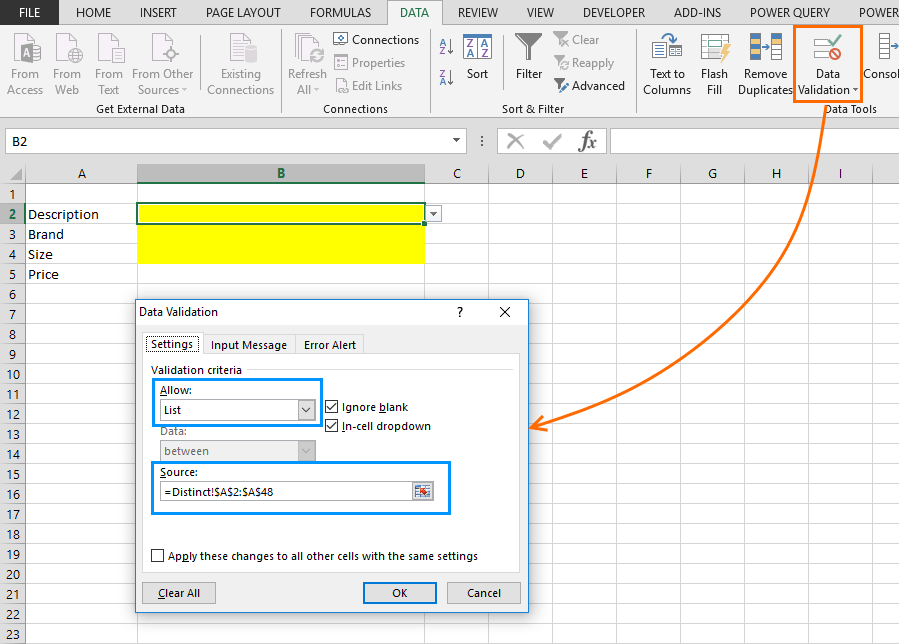
- Click the DATA tab > Data Validation.
- In the Data Validation window, select List in the Allow list.

- Select Description list with unique values.
- Click OK to create the input.


Concatenating the Dropdown Options
Next, we’re going to concatenate the first level dropdown options (Description) using the distinct list of the second level (Brand) to create a list of unique values. This will allow us to create the second level dropdown options. We will then need to create the dropdown input like we did in the previous step.

Let’s take the formula,
=Quote!$B$2&C2
Here, the absolute value cell (in $ symbol) is referencing the Description dropdown value. Note that “TENNESSEE WHISKEY” value is already selected in our example.
At this point, we’re going to create a new column for the formula that will provide us the items from our new list. The formula will match the selection with the items from our Description list. If it’s a match, this formula will return an incremental value that we’re going to use to create the second level dropdown.

=IF(COUNTIF(List!$D$2:$D$3045,D2)>0,E1+1,E1) formula will check whether items exist in all columns(the COUNTIF function does this). If the answer is yes, it adds 1 to the cell value above, if not it keeps the existing value. Note that the column header cell (E1) is left empty to prevent any errors that might be caused when there is a value in the first cell in the search list.
Lastly, we’re going to use another formula to create a list from matched values.

=IFERROR(INDEX($C$2:$C$2215,MATCH($K2,$E$2:$E$2215,0)),"")
This formula uses the MATCH function to locate the Description & Brand matches from the number list ($E$2:$E$2215) created in the previous step. It then uses these coordinates to get Brand names from the distinct Brand list ($C$2:$C$2215). The IFERROR function returns the empty values when there are no mismatches. Note that the column F ($F2 reference in formula) is used as an index value for the MATCH search.
Now the Brand list is ready and we can create the corresponding dropdown. Repeat the same steps from the Description list to create this input. Make sure to contain all possible Brands items when creating this list. Here, we selected the range (G2:G278) because “STRAIGHT BOURBON WHISKEY” has the highest number of Brands under it (277 brands).
Description, Brand, and Size

Repeat the steps for Concatenating the Dropdown Options to generate the same list for the Size parameter. Keep in mind that because this is the third level, the search value needs to be Description AND Brand AND Size. To demonstrate, “Gentleman Jack Whiskey” is selected as Brand.


We just finished creating all inputs! Finally we can get a price value from list. Since we already have a list for Description & Brand & Size combination (List!$F$2:$F$3045), we can find the price easily by searching Description & Brand & Size combination from dropdowns.

=IFERROR(INDEX(List!$D$2:$D$3045,MATCH($B$2&$B$3&$B$4,List!$F$2:$F$3045,0)),"")
In this formula, we search for Price in List!$D$2:$D$3045 range using the coordinates from the MATCH function that searches the selection (Description & Brand & Size) in List!$F$2:$F$3045 range.

And that’s all! We have successfully created a dynamic quoting tool that can be used to filter down a huge list to look up the price of a specific item. Tools like this are often used in sales to produce a quote with ease and accuracy. Although using dynamic tables can be tricky at first, you will master them in no time and utilize their full potential.
