Following certain guidelines when working in Excel can save you the headache of dealing with errors. And if something does go wrong with a formula, there are things you can still do. Let’s take a look at some recommended methods for creating formulas, and how to handle errors, should you encounter them.
Common Practices to fix a Formula in Excel
Begin Every Excel Formula with an Equal Sign (=)
Formulas typically start with the equal sign (=). Alternatively, you can begin with the plus sign (+), which will be automatically converted into an equal and plus (=+). However, this usage is only intended for backwards compatibility for Lotus 1-2-3 users. Equal and plus (=+) usage is often considered to make a formula confusing and dirty.

Match All Opening and Closing Parentheses So They are in Pairs When Writing an Excel Formula
Usually Excel won’t allow you to enter a formula without the closing brackets, and will offer you a corrected version of the formula. Auto-correct works very well with simple excel formulas.
While Excel is a powerful tool for various calculations, it may encounter limitations, particularly when dealing with intricate and lengthy formulas. In such cases, understanding how to fix formula errors in Excel becomes crucial. An essential aspect to be aware of is that Excel employs color coding to distinguish formula elements, aiding in the identification of potential errors. Paying close attention to these color codes can significantly enhance your ability to troubleshoot and correct formula-related issues. Notably, each time you open and close parentheses, Excel assigns distinct colors to the pairs. A useful tip for resolving formula errors is to move your cursor onto one of the parentheses, prompting both elements of the pair to be highlighted in bold. This visual cue is instrumental in pinpointing errors and efficiently rectifying them within your Excel formulas.

Use Quotation Marks Around Text in Excel Formulas
A common mistake encountered while creating formulas in Excel is omitting quotation marks when dealing with strings. Without these essential quotation marks, Excel attempts to interpret the entered text as a formula, reference, or named range. Consequently, this often results in the #NAME! error, indicating that the software is unable to recognize the provided text as a valid formula or reference. Fortunately, rectifying this formula error in Excel is straightforward. By ensuring proper syntax and encapsulating strings within quotation marks, users can prevent and effectively fix the #NAME! error, ensuring accurate formula execution and data processing in their spreadsheets.

Advanced Features
Use Named Ranges and Tables
In the realm of Excel data modeling, efficient navigation through vast datasets is paramount. Steering clear of direct references and embracing the power of Named Ranges and Tables can significantly elevate clarity and ease of management. Incorporating identifiers like "productlist" or "products[name]" not only enhances intuitiveness but also fosters streamlined collaboration across various tabs or workbooks, a critical need when dealing with expansive datasets.
Named Ranges prove to be a valuable asset by accommodating both references and formulas, thereby enhancing the readability and organization of your data models. Assigning Named Ranges is a straightforward process: select the desired reference(s), input a meaningful name in the formula dialog on the left, and press Enter. This strategic use of Named Ranges not only optimizes your workflow but also acts as a safeguard against formula errors, establishing a more resilient and user-friendly Excel environment.
In the context of troubleshooting, the ability to address formula errors in Excel is paramount. Named Ranges, with their clear and easily identifiable references, play a crucial role in error detection and correction. In the event of an error, the use of Named Ranges facilitates swift identification of the problematic formula, enabling efficient resolution. Mastering the art of addressing formula errors ensures that your Excel models maintain accuracy and reliability, contributing to a seamless data management experience. Discover how to fix a formula error in Excel with the precision and effectiveness offered by strategic Named Range implementation.

T
Tables stand out as superior entities compared to named ranges, particularly when handling tabular data. Their dynamic structure, coupled with advanced tools for navigating and filtering individual columns, makes them a preferred choice. Unlike named ranges, tables possess the inherent ability to expand or contract automatically based on data additions or removals.
Leveraging the power of tables in Excel not only enhances data organization but also simplifies formula referencing. When working with a table, you can easily call upon individual columns, titles, or even the entire table itself by simply typing the corresponding names. For example, inputting "Full Name" in a formula will seamlessly reference the first column below.
In the context of managing data and formulas in Excel, it's important to address potential errors that may arise. Knowing how to fix a formula error in Excel is crucial for maintaining accurate and reliable calculations. In the next section, we'll explore common formula errors and provide insights on resolving them effectively.

For more information about Named Ranges and Tables, please visit our Writing Efficient Formulas article.
Common Errors and a Workaround
Green Arrows and Formula Auditing
Excel will show a tiny green arrow at top-left corner of a cell if there is an issue with it.
Selecting the cell will display the Trace Error button (the button with exclamation mark) which will give an error description when you hover your mouse over.
Click the Trace Error button to see more information about the error and options to solve it. Clicking Help on this error will show you general guidelines for that particular error, whereas Show Calculation Steps will help troubleshoot the issue with Excel’s built-in help engine.
For more information about troubleshooting issues with Named Ranges and Tables, please see our Identifying and Analyzing Spreadsheets: Formula Auditing article.
Bypassing Errors - IFERROR Formula
IFERROR is a great way to handle errors. This formula tells Excel to do something else if there’s an error. For example, typos can cause mismatches in VLOOKUP searches and the IFERROR function will help handle those errors. IFERROR function will return a specified value when a formula returns an error.
IFERROR(value, value_if_error)
IFERROR has 2 parameters,
- value: The formula or cell reference containing the formula to be checked for an error.
- value_if_error: The value you want to return, when formula returns an error (i.e. #N/A, #VALUE!, #REF!, #DIV/0!, #NUM!, #NAME?, or #NULL!).

Visit Microsoft for further readings!