A simulation is commonly defined as an imitation of a situation or process. This typically entails creating a mathematical model that represents the characteristics and other features of a system. The model then can be used to simulate how the system will respond in certain scenarios. This can also mean forecasting or analyzing outcomes of a situation.

Although nowadays you can easily find specialized software for each use case, being a versatile calculation tool that can also store data, Excel is one of the most commonly used means to create data models and run simulations. In this article, we’re going to delve deeper into the nature of a simulation in Excel and the tools available for this purpose. You can download our sample workbook below.

The Model

A simulation in Excel must be built around a model, and that is defined by a system of formulas and mathematical operations. A simple multiplication operation can be a model, as well as a workbook full of complex formulas and macros. All that matters is the model's ability to mimic the real-time process that it’s used to solve.

Let’s take a profit calculator as an example. Companies want to know how many units of products they sold and calculate how much profit it will generate for the next year. Typically, profit is the number of goods sold times the cost of one unit, minus any costs. Let’s try to formulize this below.

= Units_Sold * ( Sell_Price - Unit_Cost )

We know the cost of a single unit, but number of units to be sold and the profit are the two unknowns in this equation. So, the next step is forecasting how many items will be sold.

The Inputs

Determining the inputs is just as important as building the calculation model. Without correct inputs, a model can’t generate the correct results. There are various ways to determine the inputs and, unfortunately, none of them are perfect. If there was a perfect way, forecasting would be a far easier analysis than it actually is.

We recommend avoiding the traditional deterministic ways that rely on some fundamental assumptions. A stochastic approach, on the other hand, will provide more reliable results. A stochastic approach is based on collecting random variables. These random variables can be used as is, or can be used to generate inputs through additional calculations.

With each run of the simulation, a new random variable is generated and used as an input. Randomness between results will decrease and become meaningful with enough number of runs. When creating a simulation in Excel you can use either one of these two formulas to generate random numbers:

RAND() returns an evenly distributed random numbers greater than, or equal to 0, and less than 1.
RANDBETWEEN(bottom, top) returns a random integer between the bottom and top parameters.

These functions return different values with each calculation. You can press the F9 key to run the calculations again in the entire workbook, and see how they act.

However, a collection of completely random values is not a real-world scenario. Instead of sending what you get from the RAND functions, you can use the results to generate numbers in a specific probability distribution. A probability distribution is a mathematical function that provides the probabilities of occurrence of different possible outcomes in multiple calculations.

Excel also has statistical functions for probability distributions. These functions can generate random input values when combined with the RAND function. Below are some of those functions.

Normal: DIST, NORM.INV
Standard normal: S.DIST, NORM.S.INV
t-distribution: DIST, T.INV
F-distribution: DIST, F.INV
Chi-square: DIST, CHI.INV
Lognormal: DIST, LOG.INV
Binomial: DIST, BINOM.INV
Hypergeometric: DIST
Beta: DIST, BETA.INV
Gamma: DIST, GAMMA.INV
Exponential: DIST
Weibull: DIST
Poisson: DIST
Negative binomial: DIST

We use a sample for normal distribution which is one of the most common distributions. The NORM.INV function returns numbers in a normally distributed fashion for the specified mean and standard deviation. The syntax of the function is like below.

NORM.INV(probability,mean,standard_dev)

To randomize the results, we use the RAND function as the probability argument. The RAND functions return value specifies the percentile of random variable with a given mean and standard deviation. Below is an example.

NORM.INV(RAND(),150,25)

The mean and standard deviation values should be consistent of expected collection of input values. For example, if you are trying to forecast next year profits, the previous year sales amounts can be used as sample data. Excel has built-in functions to calculate the mean and standard deviation.

Mean:

=AVERAGE(numbers)

Standard Deviation:

S(numbers)
P(numbers)
STDDEVA(numbers)
STDDEVPA(numbers)

Running a Simulation in Excel

So far, we covered the basics of a data model and how to create random input variables based on a probability distribution. However, stochastic simulations too can become meaningful when they are run several times. "Many" in this context, can mean 1000 or more, depending on your model. Therefore, simply recalculating the Excel workbook by pressing the F9 is not a practical way to get simulation results at this point. Let’s look at our alternatives to do this automatically.

A VBA macro can run calculations multiple times, and print the results in the workbook. Obviously, this method requires some expertise in VBA.
Third-party add-ins that can be found on the internet.
Excel's Data Table feature, especially if you have 1 or 2 input variables.

Data Table Feature

The Data Table feature is a What-if analysis tool that can calculate a formula several times based on up to 2 inputs. We can use the Data Table tools to recalculate our simulated results by tricking it with empty inputs. Let's see this on an example.

We assume a company is looking to forecast how many products it can sell, and how much profit it can make. We’re going to use the same formula we came up with before.

=Units_Sold*(Sell_Price-Unit_Cost)

Let’s examine a scenario:

The company buys the product at $8 and sells it for $12.
The mean (average) and standard deviation of units to be sold are calculated from previous sales.
A normal distribution is used to generate the number of units sold. Decimals are irrelevant because this number is generated for use as a random value in a 1000 runs.

The cell C10 contains the formula for the profit result of a single run, and this value will be the center point of the Data Table. Move the cell or use its reference in a cell that has at least 1000 empty cells below it. In our example, we used cell G2.

=C10

The next step is generating the numbers from 1 to 1000 in column F, starting from the third row. To do this:

Click the cell F3.
Go to HOME > Fill > Series.
Select Columns
Enter 1000 as Stop value.
Click

Now we are ready to use the Data Table.

Select a range that includes both the profit and numbers from 1 to 1000. In our example; F2:G1002.
Follow the path DATA > What-if Analysis > Data Table.
Click the Column input box and select an empty cell. We choose H2.
Click OK to finish the process.

Excel automatically places a special function into the empty cells named TABLE. These cells are dynamic. Each time you recalculate the workbook these cells will be updated as well, which is essentially a fast way to run another 1000 calculations.

The Results

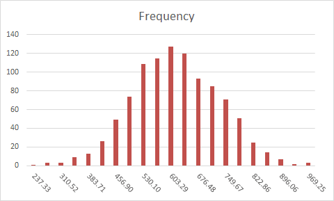
The results of a stochastic simulation can be summarized using histograms. A histogram is a representation of the distribution of numerical data. Instead of checking every simulation result, grouping them into specific percentiles can give you a better overview of the big picture.

You can create a histogram in Excel in two ways:

Analysis ToolPak add-in
Formulas

Analysis ToolPak

The Analysis ToolPak add-in is a very useful tool that shines in data analysis. It is a ‘hidden’ add-in, because it’s not active in Excel by default. You can activate it from the Add-ins dialog from FILE > Options > Add-Ins. Here, select Excel Add-ins in the Manage dropdown and click the Go button. Select the Analysis ToolPak and click OK.

The tool can be found under the DATA tab after activation with the name of Data Analysis. You will see the Histogram option in this dialog. Selecting it and clicking OK opens the Histogram window.

In Histogram dialog, Input range and Bin range should be selected. The Input range is the results of the simulation. The Bin range is the numbers that specify the limits of each interval. You can use static numbers as you need, or calculate them with formulas to make them dynamic like in simulation results. The Histogram dialog allows you to choose the target location and create a chart.

Unfortunately, the Histogram in the Data Analysis is not dynamic and you have to open the Histogram dialog every time with a new set of data.

Formula

The FREQUENCY formula can calculate the values needed for a histogram. It calculates how often values occur within a specified range. This formula also needs bins values, and the first thing we need to do is to calculate the bins.

Determine number of intervals. This is optional, but more steps increase the precision level. Too many steps might make it harder to read the results. We choose 21 for our example.
Calculate the minimum of values. =MIN($G$3:$G$1002)
Calculate the maximum of values. =MAX($G$3:$G$1002)
Calculate the difference between the minimum and maximum. =max-min
Calculate the bin size. =diff/(interval_count-1)

Now, since we know the start point (minimum value) and the bin size, we can create our bins.

The first bin is the minimum value. =min
Select the cell below and add the value above to the bin size. =K8+binsize
Copy down the cell for 20 intervals.

You can use these bins values for Data Analysis' Histogram as well. Let's move on with the FREQUENCY formula.

Start by selecting the empty range next to the bins. (L8:L28)
Type in the FREQUENCY formula, using the simulation results and bins values as arguments. =FREQUENCY(results,bins)
Press the Ctrl + Shift + Enter key combination instead of just pressing the Enter key to enter the formula.

This will create the histogram. You can see that the majority of scenarios are gathered around the middle points. This is where the most likely results lie. To see the results in an easier to read format, you can graph this data.