Although Excel already has built-in sorting features, doing this with formulas might be useful in some cases for a more dynamic approach. The formula approach will be updated automatically whenever calculations are executed. In this article, we're going to show you how to sort text in Excel using formulas.
Sort text in Excel using formulas
This is a two-step process. First, we need a helper column which will generate a sequential list of numbers and rank our data. For example, the 1st rank should be the top of the list in a sorted list. Second step is, obviously, sorting the values based on their "ranks". So, let's begin with creating the helper column.
Helper column
A "helper column" is typically created next to the actual data set, and contains formulas to generate values to be used in other calculations. There are two reasons for using a helper column here: First, you can avoid creating long and complex formulas with this, and second, you may need to use the entire column as a range in other formulas. The second case is why we choose to use a helper column in this example.
Now, let's create a helper column. We are using the COUNTIFS function to rank the text values (COUNTIF function will work too. We are using the COUNTIFS, because it's newer.). Here is the formula in the first cell of our helper column:
In this formula, shuffled represents a named range that contains the list of unsorted text. The cell B3 is the first cell of the shuffled named range. We get the helper column by copying the formula all the way down through the shuffled list.

Using the "less than or equal operator" ("<=") for a range of text values allows Excel to handle this operation by evaluating text strings based on the ASCII numbering scheme. Thus, the formula counts the values in the list (shuffled) that are less than or equal to the specified value (B3).
For example, the formula in the screenshot above counts the text values less than or equal to the text "Charizard". The formula returns 4, because there are 3 values before "Charizard": "Alakazam", "Arcanine" and "Blastoise".
Our helper column is ready, and we are ready to proceed to the next step.
Sorting text using formulas
The formula group includes 3 different functions:
First of all, the helper named range refers to the helper column (C3:C8 in our case). $E$3:E3 is an expanding reference which will add to the range when copying the function. We will get more into the details a bit later.

This example uses the INDEX & MATCH combination to populate text values in a sorted order. Briefly, the MATCH function searches the value (index from the ROWS function) in ranks (helper), and sends the position. The INDEX function returns the value at the given position in the range shuffled.
The tricky point is generating incremental values for the MATCH function that looks up these values in the helper column. The ROWS function and the expanding reference help us generate these incremental numbers. The expanding reference grows as we copy down the formula, because its first cell is anchored with the help of $ characters. The ROWS function, on the other hand, returns the count of rows in the expanding reference. This is 1 for $E$3:E3, 2 for $E$3:E4, 3 for $E$3:E5, and so on.
If you want to sort numeric values only, please see How to use Excel sort function.