This article will guide you through splitting cells, separating data, and managing your dataset efficiently. We'll focus on the 'Text to Columns' feature, a powerful tool in Excel for separating text in a single column into multiple columns, dividing data within cells, and making your data analysis tasks more straightforward. Whether you need to separate a cell in half in Excel, separate columns, or split a single cell into two rows, the 'Text to Columns' feature simplifies these tasks.
How to Split Cells in Excel
The 'Text to Columns' feature in Excel is a powerful tool that offers a wide array of options for splitting data in Excel cells. This feature is particularly useful when you have data imported into Excel that is not formatted as you need.
Step-by-Step Guide to Using Text to Columns in Excel
The 'Text to Columns' feature in Microsoft Excel is a powerful and essential tool for anyone looking to enhance their data management skills. This feature excels at splitting cells in Excel, a task often encountered by users who must reformat data imported from various sources.
- Preparation for Data Splitting: If you aim to separate text in Excel cells into two, look for natural separators in your data, such as commas or tabs, which are common in imported data.
- Activating the Feature: Found under the DATA tab, the 'Text to Columns' icon is your gateway to separating and organizing your data. It's a feature when you need to separate Excel cells into multiple rows or manage complex data sets.
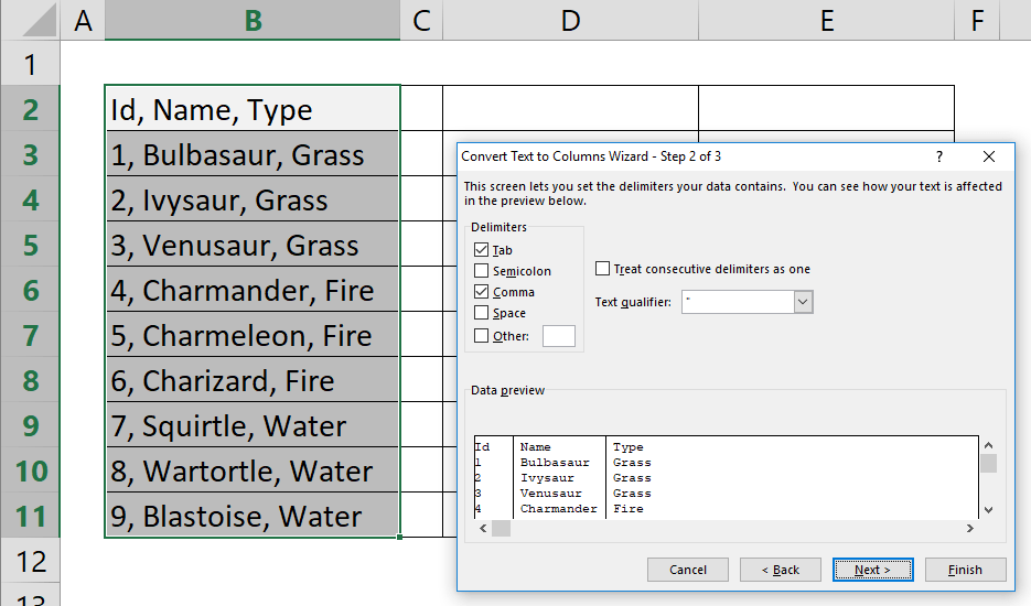
- Selecting Separation Method:
- Delimited Split: This method is perfect for data separated by characters (like commas, semicolons, or spaces). It's particularly useful for separating data in Excel, where each piece of information is distinctly marked by such separators.
- Fixed Width Split: Choose this method when each data segment in your cell has a fixed length. This approach is ideal for evenly separating data across multiple cells or splitting a single cell in Excel into equal parts.
- Fine-Tuning the Split:
- Delimited Mode Adjustments: Here, you can specify multiple delimiters. This feature is very helpful when dealing with complex data structures, such as splitting a cell in Excel that contains a mix of different types of information.
- Adjusting Fixed Width: You can control how to separate your data by setting specific column widths. This control is critical for tasks like splitting a cell in Excel into two or more specific sections.
- Formatting the Resultant Data: Excel provides options to format each new column created. This step is crucial for maintaining data integrity when you split cells in Excel, ensuring that numerical and date data types are correctly interpreted.
- Completing the Data Separation: Once you set the destination for your newly organized data and click 'Finish,' Excel will execute the separation. This action can transform a single, cluttered column into a well-organized data set, whether you're looking to split columns in Excel, separate information within a cell, or separate a cell diagonally in Excel for visual effect.
- Beyond Basic Splits: 'Text to Columns' is not just limited to simple splitting tasks. It can be used in advanced ways, like when you need to separate text in Excel cells by space, separate names in Excel into two columns, or even split data in Excel cells for analytical purposes.
- Practical Applications: The practical applications of 'Text to Columns' are vast. For example, you can use it to split a name field into first and last name columns, divide a lengthy address into separate components, or even separate text in an Excel cell into two columns for better data visualization.
The 'Text to Columns' feature is an invaluable asset in Excel. It provides solutions for a wide range of scenarios, from splitting a cell in half in Excel to splitting one cell into multiple rows and even separating data in Excel from one cell. Mastering this feature can significantly streamline your data processing tasks, making your work with Excel more efficient and effective.