Excel already has functions like the SUMIF and the SUMIFS for summing data by groups. However; they can't work if you have date-time values combined. This article shows How to sum by date in Excel without time using SUMPRODUCT and INT functions.
Syntax
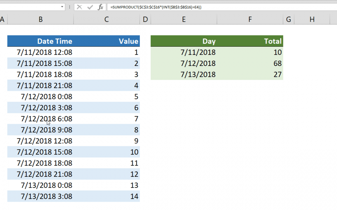
=SUMPRODUCT( range of values * ( INT( range of date-time ) = cell of date ) )
Steps
- Start with =SUMPRODUCT( function
- Type of select the range that contains values $C$3:$C$16
- Use asterisk to product range values with condition range and open a parenthesis *(
- Continue with INT($B$3:$B$16) to remove the time part
- Enter condition with an equal sign and criteria range =E3
- Type )) to close function and finish the formula
How to sum by date in Excel
Excel keeps date and time values as numbers. Excel assumes the history starts from Jan 1st, 1900 and accepts this date as 1. While whole numbers represent days, the decimal represents time. For example, 1/1/2018 is equal to 43101, 12:00 is equal to 0.5.
We can use the INT function to get rid of the time values or decimal part of numbers. The INT function simply returns the whole number part from a numeric value. In our case;
INT($B$3:$B$16) returns {43292;43292;43292;43292;43293;43293;43293;43293;43293;43293;43293;43293;43294;43294}
However; to make the INT function work on an array, we need to use the SUMPRODUCT function. The SUMPRODUCT function’s ability to handle arrays without using array formulas provides an advantage over the limitations of SUMIF and SUMIFS functions. The SUMPRODUCT can evaluate and return arrays from range – value conditions. We use this functionality to resolve criteria range – criteria pairs.
(INT($B$3:$B$16)=E3) returns {TRUE;TRUE;TRUE;TRUE;FALSE;FALSE;FALSE;FALSE;FALSE;FALSE;FALSE;FALSE;FALSE;FALSE}
Also, the SUMPRODUCT function sums the values in its argument array if there is only one argument. However, conditional equations returns Boolean values. So, they need to be converted to numbers which are meaningful for the SUMPRODUCT function. Fortunately, the product operator (*) does this.
By multiplying a value array with a condition array, we get the array values generated according to our needs.
$C$3:$C$16*(INT($B$3:$B$16)=E3) returns {1;2;3;4;0;0;0;0;0;0;0;0;0;0}
Finally, the SUMPRODUCT returns the results as sum by date in Excel which is what we are looking for.
=SUMPRODUCT($C$3:$C$16*(INT($B$3:$B$16)=E3)) returns 10 for the date of 7/11/2018.
Alternative Option
An alternative way is using PivotTable that can give you more options than summing values. You can find detailed information in How to group days without time by Pivot Table.
Also see related articles how to calculate weighted average with SUMPRODUCT, how to SUM 2d ranges with SUMPRODUCT, and how to sum values with OR operator using SUMPRODUCT with multiple criteria.